
Location
 FR
FR
Badges
Activity
Challenge Categories
Challenges Entered

Play in a realistic insurance market, compete for profit!
Latest submissions
See All| graded | 127171 | ||
| failed | 127155 | ||
| failed | 127152 |
| Participant | Rating |
|---|
| Participant | Rating |
|---|
Insurance pricing game

You are probably wondering how much profit loading to select?
About 5 years ago@alfarzan this is interesting ; in another thread ( “Asymmetric” loss function? ) we discussed how the optimal margin strategy of a player depends on the quality of his own estimate ; as @Calico suggested, more unknown in the estimate probably lead to higher optimal margins.
Here you get an opposite approach and conclude that the margin should not depend of the variation of your own estimate but on the variation of your competitors estimate…
And in both case, more uncertainty leads to optimal strategies with higher margin.
This topic definitely deserves more serious investigation !
Sharing of industrial practice
About 5 years agoI have been a pricing actuary for a few years and can give you what I saw in different companies. I may lack objectivity here, sorry in advance 
Here is what I see for risk modeling in pricing:
-
GLMs : (Generalized Linear Models) : prediction(X) = g^{-1}(\sum_d \beta_d \times X_d) - with possible interactions if relevant. g is often a log, so g^{-1} is an exponential, leading to a multiplicative formula.
Here all the effects are linear (so of course it does not work well as soon as one wants to capture non-linear effects such as in an age variable). Below 2 example - one good and one bad - with the observed values in purple and the model in green:
It is possible to capture non-linearity by “extending” the set of input variables, for instance by adding transformed version of the variables in the data-set - so one would use age, age^2, age^3… or other transformations to the data-set to capture non-linearities. This is very very old-school, tedious, error-prone, and lacks a lot of flexibility. -
GAMs : (Generalized Additive Models) : prediction(X) = g^{-1}(\sum_d f_d(X_d))) : the predictions are the sum of non-linear effects of the different variables ; you can enrich the approach by including interactions f_{d,e}(X_d,X_e) if relevant.
The very strong point of this approach is that it is transparent (possibility for the user to directly look into the model, decompose it, understand it, without having to rely on analysis / indirect look - eg PDP, ICE, ALE, …) and easy to put top productions (the models are basically tables). So they are a powerful tool to prevent adverse-selection while ensuring the low-risk segments are well priced, and are often requested by risk-managements or regulators.
However these models were often built manually (the user selects which variables are included, what shape the functions have - polynomial, piece-wise linear, step-functions, …) either through proprietary softwares or programming languages (eg splines with Python / R). For this reason GAMs are often opposed to ML methods and suffers from a bad reputation.
Newer approach allow the creation of GAM models through machine learning while keeping the GAM structure (I believe Akur8 leads the way here - but I may lack some objectivity as I work for this company ). The idea is that the ML algorithm builds the optimal subset of variables and the shape of the f_d functions to provide a parsimonious and robust model while minimizing the errors, removing all the variables or levels that do not carry significant signal. The user runs grid-searches to test different number of variables / robustness and pick the “best one” for his modeling problem. “Best one” being the models that maximize an out-of-sample score over a k-fold and following several more qualitative sanity-check from the modeler.
For instance below a GAM fitted on a non-linear variable (driver age):
-
Tree-based methods (GBMs, RF…) : we all know these well ; they are associated with “machine-learning”, there are very good open-source packages (SKLearn, xgboost, lightGBM…), and it is relatively simple to use them to build a good model. The drawback is that they are black-box, meaning the models can’t be directly apprehended by a user - so the models need to be simplified through the classic visualization techniques to be (partially) understood. For instance below an ICE plot of a GBM - the average trend is good but some examples, eg in bold, are dubious:
-
No models : a surprisingly high number of insurance companies do not have any predictive models to compute the cost of the clients at underwriting and don’t know in advance their loss-ratios. They would track the loss-ratios (claims paid /premium earned) on different segments and their conversions, trying to correct if things go too far off-track.


I have seen many firms in Europe, where a very large majority of insurers use GAMs ; most of them use legacy solutions and build these GAMs manually ; a growing share is switching to ML-powered GAMs (thanks to us  ).
).
There is a lot of confusion as insurers tend to use the term “GLM” to describe both GLMs and GAMs.
A minority of insurers - usually smaller and more traditional ones - use pure GLMs or no models at all.
Many insurers considered using GBMs in production but did not move forward (too much to lose, no clear gain) or leverage only GBMs to get insights relevant for the manual productions of GAMs (for instance identifying the variables with highest importance or interactions). I have heard rumors of some people did move forward with GBMs but didn’t hear about anything very convincing.
In the US the situation is a bit less clear, with a larger share of insurers using real old linear GLMs with data-transformation, some using GAMs and rumors on GBMs, either directly or as scores that enter in GLM formulas. The market is heavily regulated and varies strongly from one state to another, leading to different situations. In Asia (Japan, Korea…) I met people starting to use GAMs ; the market is also very regulated there.
You are probably wondering how much profit loading to select?
About 5 years ago“Taking that to the extreme would mean a margin of zero (infinitesimally).”
For this the competitors would need to share their definition of “margin”… so they would need to have the same cost estimates for the policy .
If they don’t, the result seems far less obvious to me.
"Asymmetric" loss function?
About 5 years agoThanks @Calico that’s really nice
I wanted to dig into this topic a bit for years; this forum gave me the opportunity to do so
So I tried to model what the optimal strategy would be and how it changes based on the uncertainty in the model.
I used a very simplistic framework to try to keep things clear.
I supposed :
- there is an (unknown) risk attached to a policy, called r (say, r=100). The insurer has an estimate of this risk, following a gaussian around it : \hat r=Normal(r, \sigma) .
- there is a known demand function depending on the offered premium \pi : d(\pi) = logit(a+b \times ln(\pi))
In this situation, the first conclusions can be derived :
- for every price \pi a real profit B(\pi) can be computed (but it is unknown to the insurer as the real risk r is unknown : B(\pi)=d(\pi) \times (\pi - r) ).
- an approximation of this real profit can be computed : \hat B(\pi)=d(\pi) \times (\pi - \hat r) ; interestingly it is an unbiased estimate (but using it for price-optimization purpose very quickly lead to funny bias ; I won’t focus on this here)
- it is quickly clear that most of the computations we can do will not lead to a closed formula ; the reason for that is because the real optimum (solving \dfrac{dB(\pi)} {d\pi}=0 ) does not lead to an explicit solution, I think. So all the results here will be based on simulations.
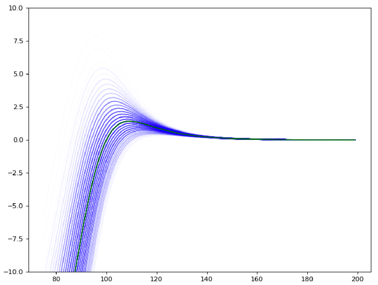
For instance in the graph below (x axis : premium \pi ; y axis : expected real profit B(\pi) - in green - or estimated profit \hat B(\pi) in blue, for different values of \hat r) provides an view of the truth and the estimated truth according to the model.
The question raised by @simon_coulombe is : given an estimated risk \hat r and a known variance in this estimate \sigma, what is the best flat-margin (called m) to apply, in order to maximize the expected value of the real profit : m^*=argmax_m E(B(\hat r \times (1+m))) ?
The intuition we all shared is that it should increase with \sigma. @Calico suggested it should be linear.
As there is no obvious formula answering this question, I ran simulations, taking an example of demand function (a=64, b=-14), a real r (100), and varying \sigma, running 1000 simulations with different \hat r every time.
For every value of sigma, all values of the margin m were tested and the one driving the highest profits B(\hat r \times (1+m)) on average over the 1000 simulations of \hat r was found.
The optimal margin m increases as expected when \sigma increases, as one would expect :
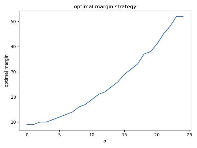
(the values are rounded and there is some noise around \sigma = 20 but it looks more or less linear, indeed).
The profit goes this way :
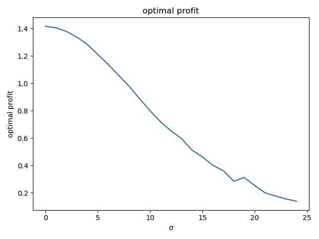
(if the real risk r is exactly known - \sigma = 0 -, a profit of 1.42 can be obtained. If \sigma goes to infinitly large values, the profits tends toward zero.)
This simple test raises a lot of questions that I would like to investigate more seriously in the future :
- is the optimal margin really linearly increasing with \sigma ?
- if I use a noise that is not gaussian, what will be the relation ? Maybe there is a distribution of the errors that helps the maths ?
- in this toy example, the demand function was supposed to be known ; what happens if it also contains errors ?
- how can I estimate the model errors (it is very hard for the risk models, but probably much harder for the demand and price-sensitivity models !!)
- strategies optimizing naively the estimated profits \hat B(\pi) built from the estimated risk \hat r are known to be a bad, leading to over-estimated profits and suboptimal pricings ; can a simple correction factor be applied, and how does it relate to \sigma ?
So to summarized, this test kind of confirms the intuition is more or less true, but opens many more questions !! If anyones has some papers on this topic, I would be really happy to get more serious insights !
"Asymmetric" loss function?
About 5 years agoThat’s a great topic !!
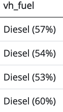
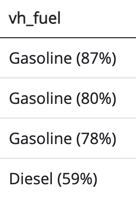
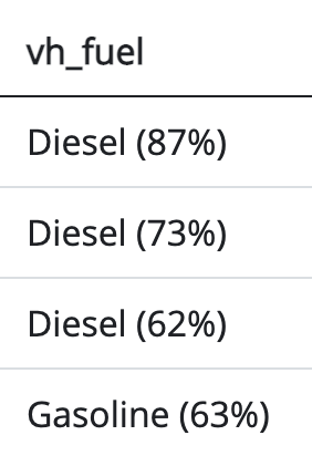
During the competition I did something similar to you, for instance on the vehicle IDs, I decided to “cap” all the effects below -5% (and refitted the model) as illustrated for some vehicles in the graph below:
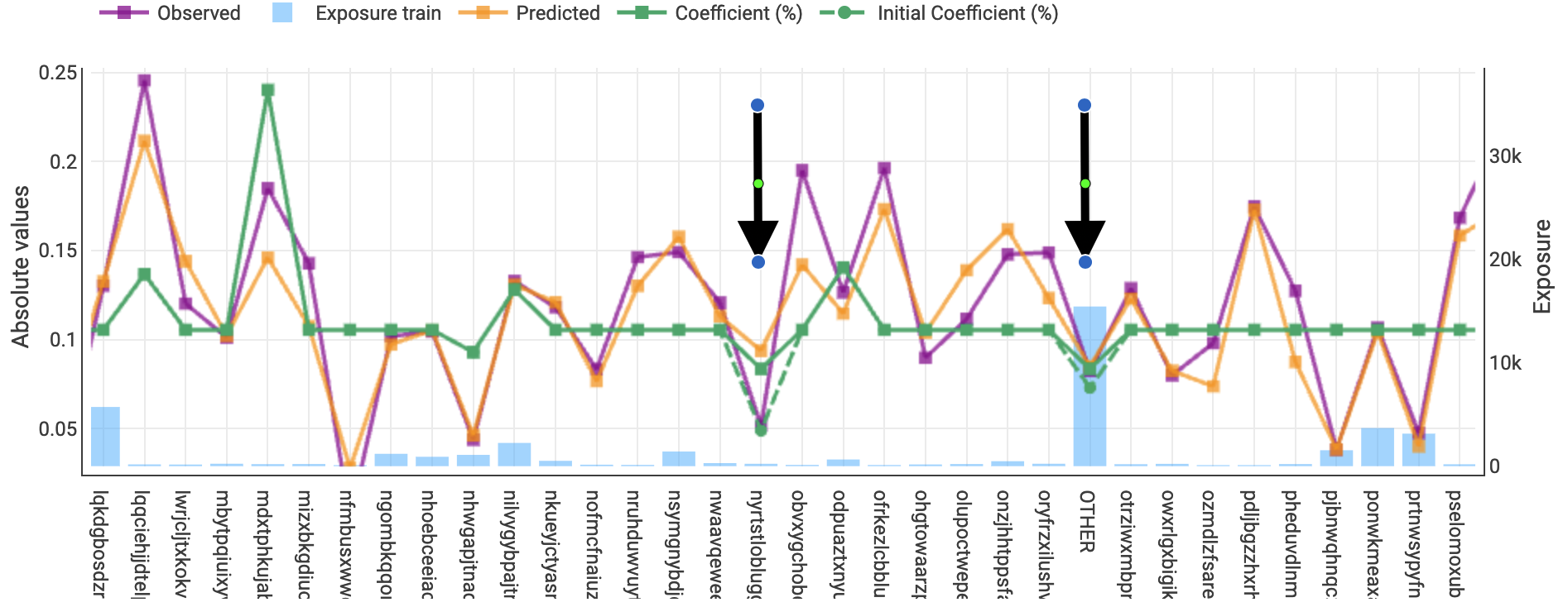
The dashed green line represents the “optimal” coefficients in term of predictiveness while the full line represents the coefficient in the model used in the pricing ; for the two levels with the arrows, the “statistical” model was having effects stronger than -5% (dashed line) but I capped the effects at -5% (full line).
This is just a very dirty actuarial cooking but the idea is the same as you : “in case of doubt, I am happy to increase the price but not happy to decrease it”.
A cleaner approach (where you assess the variance of your predictions for each profile and charge a buffer depending on it) would clearly be much better but I don’t know any research on this ; I don’t have a clear motivation for this approach, providing a formula for this buffer. Does someone know any paper with a real, rigorous and formal version on this topic ?
Margins & Price Sensitivity
About 5 years agoThanks @Calico for sharing your approach! I tried (like many others) to test different ranges between rounds but got discouraged when I saw people who didn’t update their submissions were going up and down the leaderboard ; really cool to use them to get a baseline !
It is also fun to see that, at the end, you targeted a conversion rate very different from mine (5% for you vs 10% for me)… and we might both miss our target given how much the market will vary in the last round 
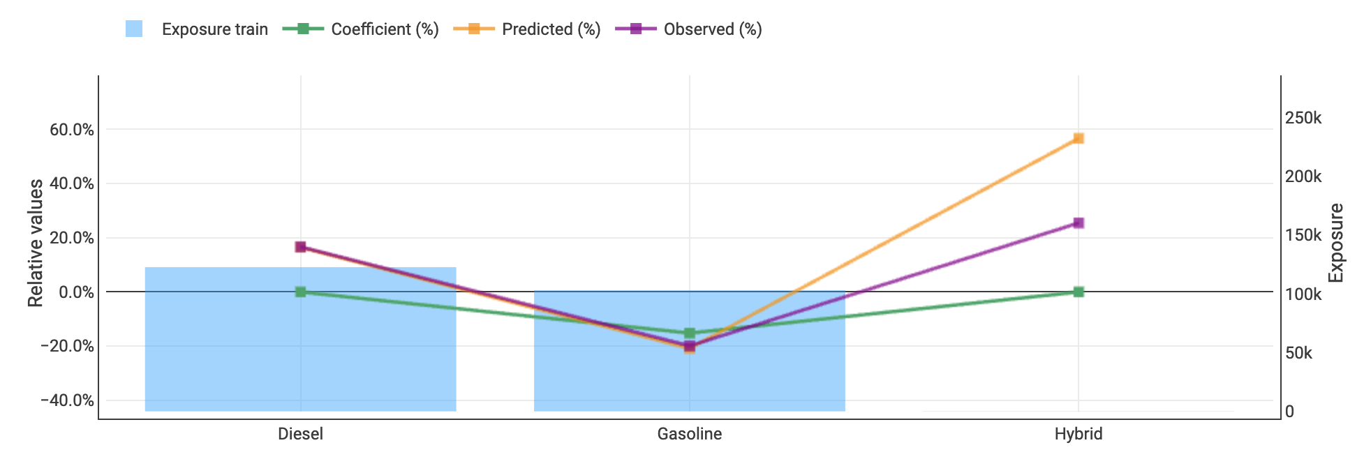
@kamil_singh the graph with fuel type on the x-axis and the relativities on the y axis was created with Akur8 ( https://akur8-tech.com/ ) actuarial modeling and pricing solution (I work for the company developing it… and it is a great pricing platform, of course ! )
@chezmoi : in general I would clearly say that demand models need a good and well identified price-sensitivity component to provide actionable results (and it brings really huge value). But here it was clearly a futile experiment, mainly for fun. While my estimates may be true for the week 10 market, it will not be for the final one, given how much the competition premiums changed. It also provide no clear vision on the individual conversion rate and behavior, as you point out.
Margins & Price Sensitivity
About 5 years agoThanks !
Some remarks & answers :
-
As you guess, the results of this study were a bit useless:
- the market is moving too quickly to leverage the results ; the results are true for one week, but the market will have shifted for the following leaderboard.
- while I guess everyone agrees that a good market share is somewhere between 5 and 15%, we can’t really optimize the prices (as we don’t really know the importance of the anti-selection effect… but if you have smart ways to leverage these results I would be really curious).
-
@simon_coulombe: I could have used a variable with more levels but then the exposure in each level is lower, so the noise is higher… (it is already very high) plus the kind of feedback we get, with only the most written level, doesn’t help for this. So I kept it simple : it is already a very rough estimate !!
-
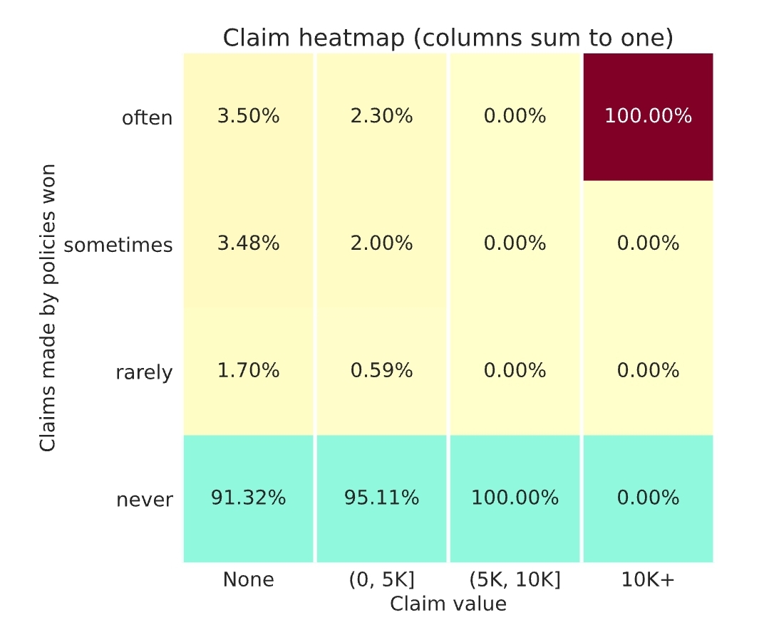
@kamil_singh: I just used a good old spreadsheet to compute these values. I computed from the conversion matrix the share of policies within each conversion category (“often” / “sometimes” / “rarely” / “never”). We also had the conversion rate in each category. So I could get the number of converted policies in each category. I could also get, in each category, the split between both fuel values, and assumed the number of each fuel & conversion category converted policies was just the product. Then I summed the conversion (for each fuel) between all the categories, and could get the number of conversion for each fuel. Finally I divided by the number of policy for each fuel and get the two conversion rates… and could draw the curves.
So as you can see it is full of simple assumptions / simplifications
So that was a funny study, and it was good to confirm that there was a lot of noise in the conversion, but the results were really imprecise I eventually decided to pick a flat margin of 25% but that was really a random pick !
Maybe one reason why the conversion was so noisy is related to the 2-step validation used during the competition. This has 2 effects :
- on the 1st round, there are a lot of “kamikaze” insurers, providing very random and low price. So in this case anti-selection plays very strongly and everyone loses money => the “best” ones are those who lose the less, ie the ones with the highest prices. That would explain why the prices are so high in the 2nd round (and, as a snowball effect, for all the players high in the leaderboard).
- the two stage scoring also ment that the “markets” only contained 20 players or so, which ment that if one or two players changed their behavior this would impact a lot the final score ; and, if the previous point is right and the “top players” of the first round included many competitors who were finding themselves with high margins then it means these players might change a lot their pricing behavior in the next round, changing the conversion profiles.
I would also be curious to see “real” graphs estimating this effect
Anyway, it was a really cool game ! Thanks @alfarzan & team !
Margins & Price Sensitivity
About 5 years agoHi everyone,
I create this thread to discus the loading strategies and price sensitivity studies you ran during the game.
@simon_coulombe described his attempt to create random shock on his margin (but didn’t receive enough feedback to leverage it  ). I also hoped @alfarzan would give us this feedback (would have opened many possibilities) but it would have created unfair information for those who joined the competition early…
On my side I tried the following strategy :
-
I took a variable which was not very relevant (vehicle fuel) and well balanced. I guessed everybody would capture its effect correctly :
-
On week 8, I used the “fair price” to both types of fuels, and confirmed my underwriting results followed the train data distribution.
-
On week 9, I gave a 10% price increase to the diesel vehicles (keeping gaz untouched). In the weekly feedback I got a very strong difference in the underwriting results.
-
To be sure, I did the same on week 10 (this time decreasing diesel, still leaving the gaz at the same price).
Finally I used these results (combined with the size of each conversion levels, the average conversion in each level, and the number of vehicles in each category) to estimate the conversion rate for each vehicle and, then, the impact on the 10% increase or decrease on the conversion. So I could finally build a conversion model for each round :
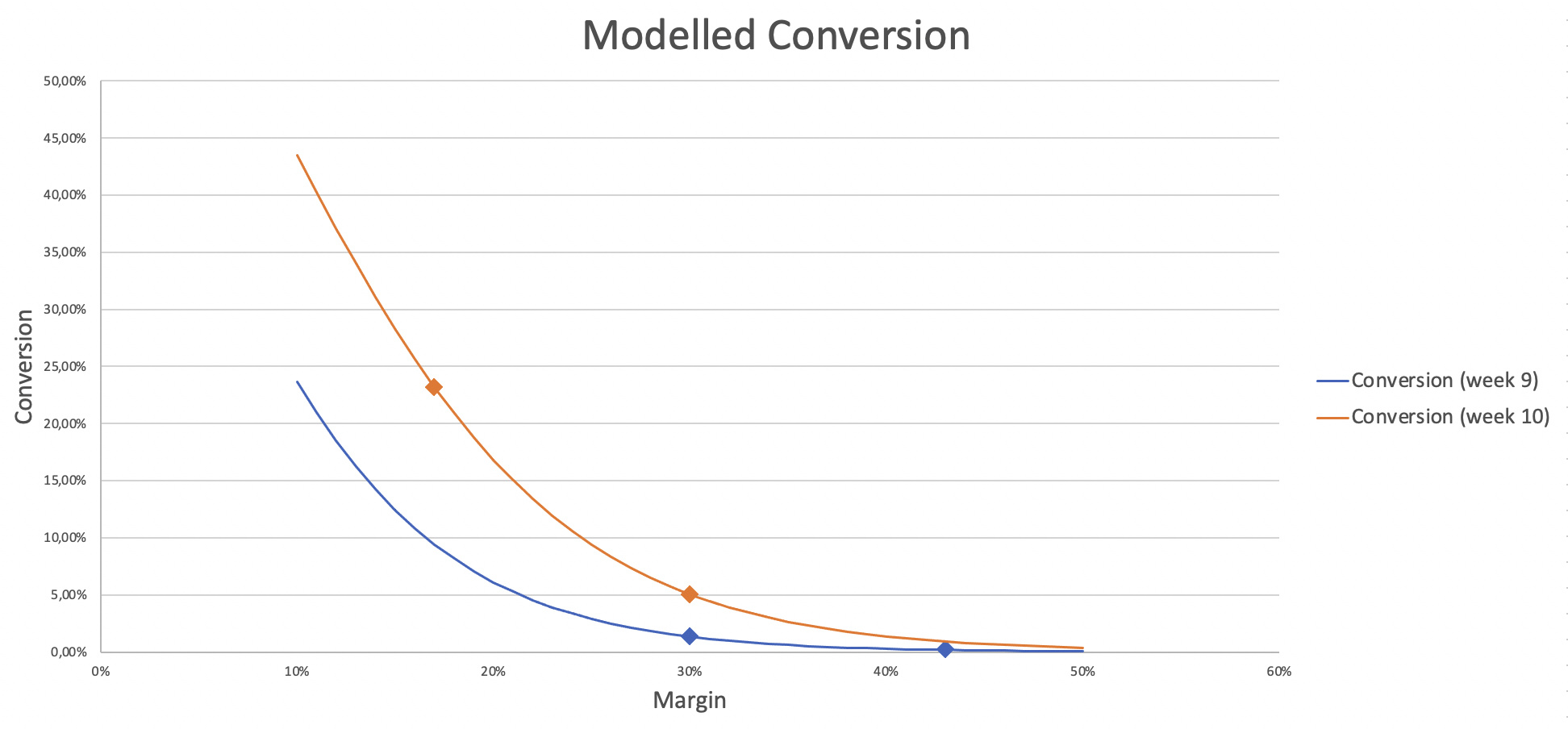
2 main conclusions out of my “demand model” :
- the elasticity of our markets are very large (above 15) which makes sense in a winner takes all environment
- the market shifted by about 7% between weeks 9 and 10, which led to very different conversion results at the same price. This instability creates a huge element of luck in the results (this is coherent with what we saw on the leaderboard, with some ranks changing dramatically while the submissions were not edited).
@alfarzan has the real data to compute this kind of curves, and it would be interesting to know what they really look like - my computation is full of ugly approximations !!!
Did anyone else try to estimate these elements of the market ?
Was week 9 a lucky no large claims week?
About 5 years agoThanks @alfarzan for your explanation, but I must say I am still a bit lost.
Taking your toy example with 10K claims, with a 10% frequency, and ignoring the last 2 columns which are very rare.
- The policies won “often” represent 3.5% of the policies with no claims - around 3.5% x 9K = 315 - plus 2.3% of the policies with a small claim - around 2.3% x 1K = 23 - so the total here is around 338.
- The policies won “rarely” represent 1.7% of the policies with no claims - around 1.7% x 9K = 153 - plus 0,59% of the policies with a small claim - around 0.6% x 1K = 6 - so the total there is around 159.
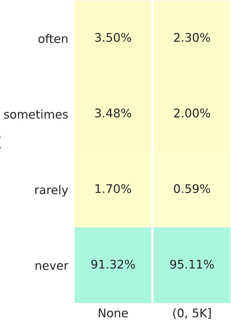
There are some approximations here, but overall, as the two values for “often” are larger than both values for “rarely” I don’t see any solution where the number of policies are equal… so I might be misinterpreting the heatmap somehow
Was week 9 a lucky no large claims week?
About 5 years agoThanks @alfarzan for confirming.
Here what puzzles me is that on all claims segments the “often” figures are much higher than the “rarely” ones. I don’t think these figures would be possible with the same number of policies in each row.
Was week 9 a lucky no large claims week?
About 5 years agoThese NaN are very strange…
I think (as pointed out by @nigel_carpenter) the results are very sensitive to the large claims…
On my side the last week results indicate one large claim around 15K that I got (relatively) often :
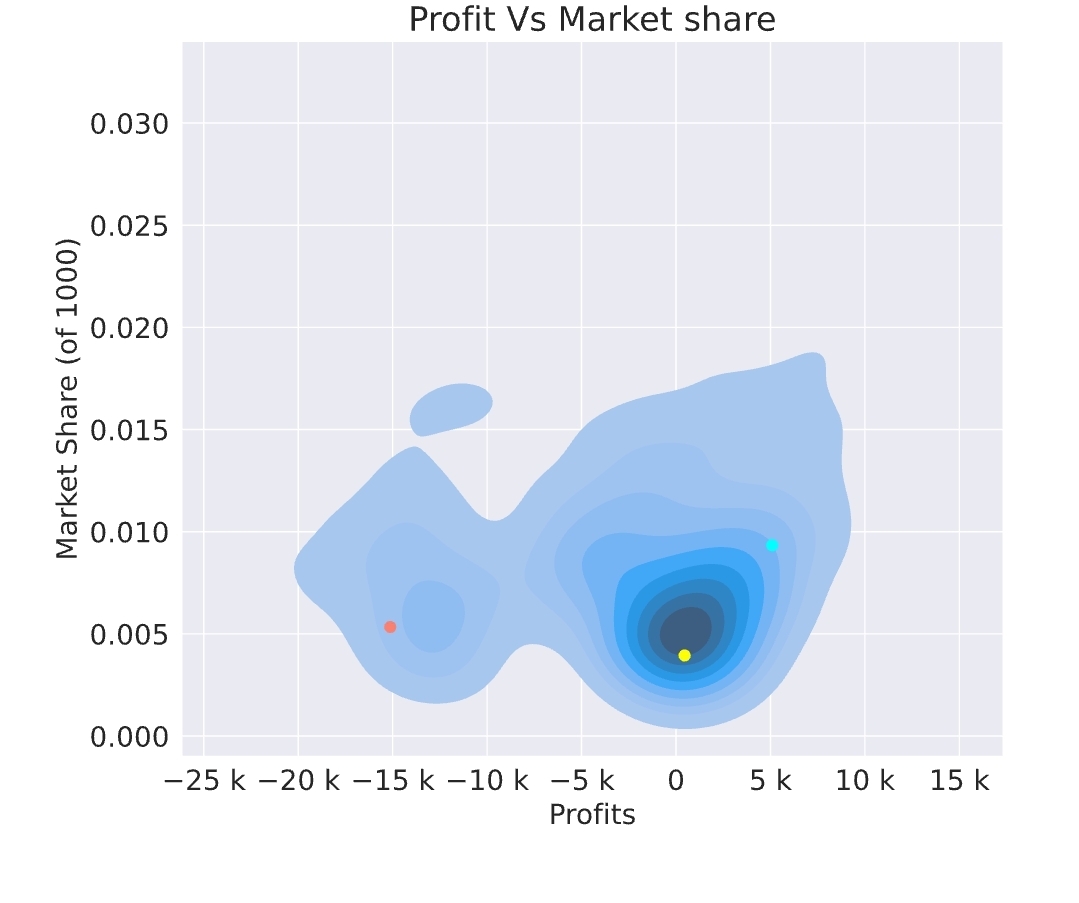
It also looks like the conversion rate still varies a lot (so the prices haven’t stabilized yet).
I have a question for @alfarzan: can you confirm the number of policies in the often, sometimes and rarely is the same ? I don’t understand how I got this split if that’s the case …
Week 7 feedback (and some thoughts)
Over 5 years agoThanks @alfarzan for these explainations.
One additional reason for the higher stability of real market is the better underwriting knowledge : insurers know on which segments they have high / low conversion rate, and have some idea of their competitors price. This feedback loop plays a major role to help the prices “converge” and stabilize.This feedback is not available here, as the weekly feedbacks provide (I believe) very insufficient conversion information. This is a reason why I would suggest a per-profile conversion rate. Other information like sharing the players profit-margins and market shares (which would be more or less public information in the real world) would also help stabilizing the market… if it is still time to do so before the final week.
Ideas on increasing engagement rate
Over 5 years agoHi @alfarzan
First of all, congrats for the work done ! It is really hard to run this kind of competition
If I can suggest way to get stronger involvement:
- For the first submissions, submitting a code and not directly the prices for known profiles makes things much harder. I think this has been strongly improved since the beginning of the competition.
- Then, the randomness of the rankings due to large claims probably discouraged a few (at least it was discouraging me) ; I think this has been solved by capping large claims / including reinsurance, which is great !
- Finally, I feel that once the players have a relatively good prediction algo, they are playing blindly on the margin they should use for each clients. I personally feel a bit stuck on how to improve my pricing strategy. Providing more feedbacks (in particular the profiles & conversion rate for the quotes in the weekly leaderboards) would, I believe, re-launch the interest of the game.
These points are not new, but I am curious to know how much the last frustration is shared by the other players.
Thanks again for organizing all this !
Week 2 leaderboard is out! Comments and upcoming feedback
Over 5 years agoHi @alfarzan
I just sent you an email with the code.
Guillaume
Week 2 leaderboard is out! Comments and upcoming feedback
Over 5 years agoHi @alfarzan
Thanks for these additional insights.
Can I ask if you could include the Tweedie likelihood and the Gini index to the feedbacks ?
This is mainly by curiosity, to see how these metrics relate to the final profit.
(if it can help, I can provide python codes for these).
Thanks !
The first profit leaderboard is out! Some comments
Over 5 years agoHi @alfarzan
Yes having the list of the profiles and, for each profile, the “conversion rate” (% of the markets in which we were the cheapest) and (optionally) the observed claims would have a huge impact on the game !
Can you clarify what the markets and the participation rates are?
Over 5 years agoHi Simon
I think the “5% rule” is a bit different : you need to get one policy in 5% of the markets :
" Participation rule. Your model must participate (i.e. win at least 1 policy) in 5% or more of the markets it is placed in."
So the 2 examples you gave do not create any issues with this rule.
Still I would also be very curious to know more about our market performance (market size, market share, offered / written premium & margin, …) to adapt our margin strategy !
Sharing of industrial practice
About 5 years agoThanks @davidlkl !
Yes this area of research is quite active (“interpreting” a black box is nice, building a transparent one from the beginning is better).
I didn’t know about the HKU work: thanks for sharing!