Seismic Facies Identification Challenge
[Explainer] - EDA of Seismic data by geographic axis
Here’s my EDA notebook on how the seismic data varies by geographic axis, along with some ideas for training.
 dipam_chakraborty


EDA on variation by geographic axis
Here’s my EDA notebook on how the seismic data varies by geographic axis, along with some ideas for training.
A peek some of the stuff in the notebook
How the patterns look per label:
How the facies vary by z-axis
Splitting the data for training based on the EDA results
Do share your feedback. 
AICrowd Seismic Facies Identification Challenge
https://www.aicrowd.com/challenges/seismic-facies-identification-challenge
The goal of the Seismic Facies Identification challenge is to create a machine-learning algorithm which, working from the raw 3D image, can reproduce an expert pixel-by-pixel facies identification.
Problem description: 3D image Semantic Segmentation
Setup Environment 📚
import numpy as np
import matplotlib.pyplot as plt
%matplotlib inline
Domain knowledge 💡
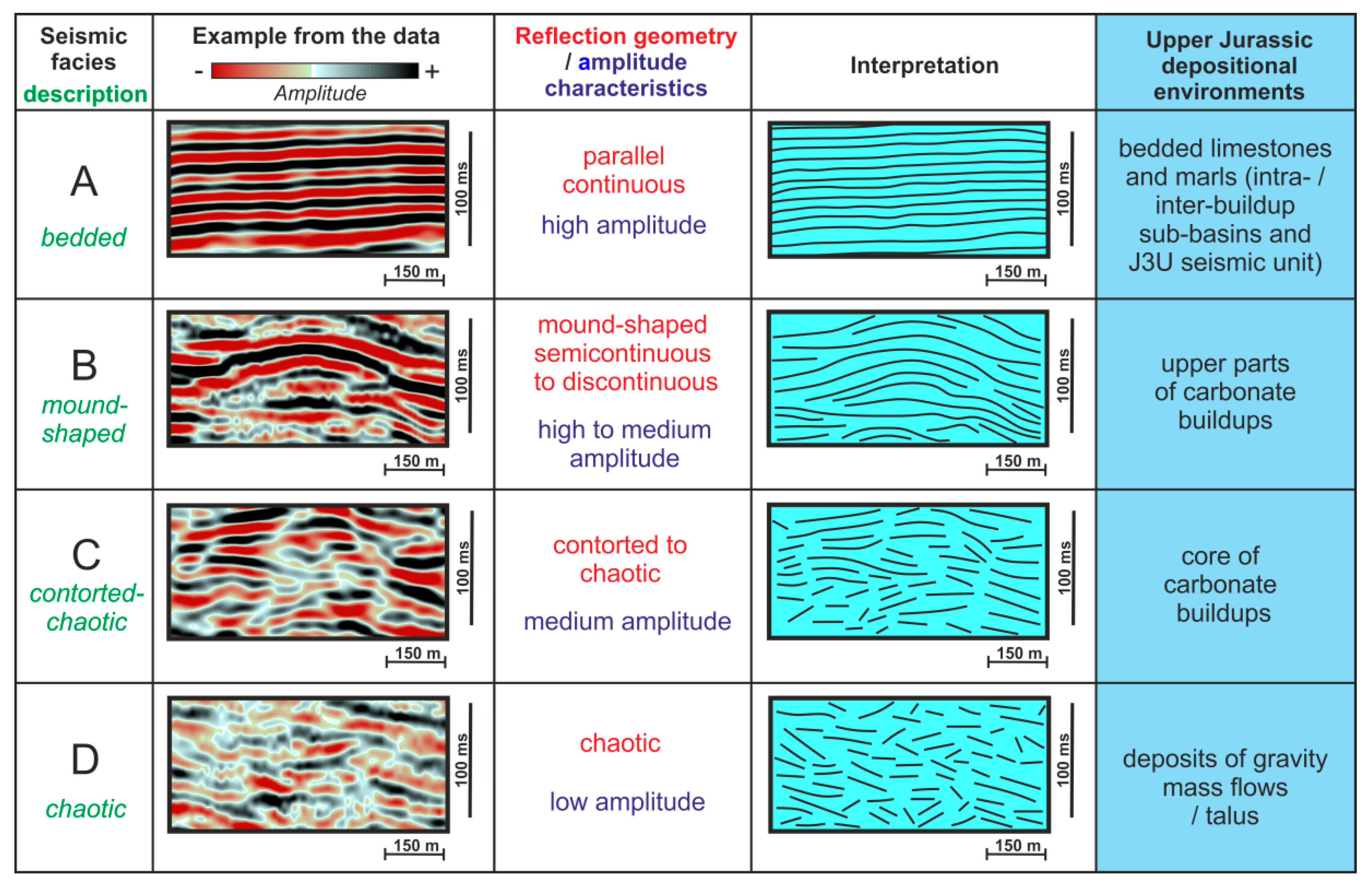
The following are the geologic descriptions of each labels:
1 : Basement/Other: Basement - Low S/N; Few internal Reflections; May contain volcanics in places
2 : Slope Mudstone A: Slope to Basin Floor Mudstones; High Amplitude Upper and Lower Boundaries; Low Amplitude Continuous/Semi-Continuous Internal Reflectors
3 : Mass Transport Deposit: Mix of Chaotic Facies and Low Amplitude Parallel Reflections
4 : Slope Mudstone B: Slope to Basin Floor Mudstones and Sandstones; High Amplitude Parallel Reflectors; Low Continuity Scour Surfaces
5 : Slope Valley: High Amplitude Incised Channels/Valleys; Relatively low relief
6 : Submarine Canyon System: Erosional Base is U shaped with high local relief. Internal fill is low amplitude mix of parallel inclined surfaces and chaotic disrupted reflectors. Mostly deformed slope mudstone filled with isolated sinuous sand-filled channels near the basal surface.
According to the literature, the facies are identified using the curves in the readings
📌 Remember
The curves seems to be low level to mid level features, so a majority of the prediction likely depends on that, but the broader context may also help
Load data 💾
# Downloading Data
!wget https://datasets.aicrowd.com/default/aicrowd-public-datasets/seamai-facies-challenge/v0.1/public/data_train.npz
# Download Labels
!wget https://datasets.aicrowd.com/default/aicrowd-public-datasets/seamai-facies-challenge/v0.1/public/labels_train.npz
# Download Labels
!wget https://datasets.aicrowd.com/default/aicrowd-public-datasets/seamai-facies-challenge/v0.1/public/data_test_1.npz
train_full = np.load('data_train.npz', allow_pickle=True, mmap_mode='r')["data"]
labels_full = np.load('labels_train.npz', allow_pickle=True)["labels"]
test = np.load('data_test_1.npz', allow_pickle=True)["data"]
A tiny peek at the data ❕
fig, ax = plt.subplots(1,3, sharey=True);
fig.set_size_inches(20, 8);
fig.suptitle("2D slice of the 3D seismic data volume", fontsize=20);
yc = 100
print(np.unique(labels_full[:, :, yc]))
ax[0].imshow(train_full[:, :, yc], cmap='terrain');
ax[0].set_xlabel('X Axis: West - East', fontsize=14);
ax[0].set_ylabel('Z Axis: Top - Bottom', fontsize=14);
ax[1].imshow(labels_full[:, :, yc]);
ax[1].set_xlabel('X Axis: West - East', fontsize=14);
ax[2].imshow(train_full[:, :, yc], cmap='terrain');
ax[2].imshow(labels_full[:, :, yc], alpha=0.4, cmap='twilight');
ax[2].set_xlabel('X Axis: West - East', fontsize=14);

EDA on images 📷
## Data histogram, min, max, mean, std
tr_ravel = train_full.ravel()
minval, maxval, mean, std = np.min(tr_ravel), np.max(tr_ravel), np.mean(tr_ravel), np.std(tr_ravel)
print('Min: %0.4f, Max: %0.4f, Mean: %0.4f, Std: %0.4f' %
(minval, maxval, mean, std))
hist = plt.hist(tr_ravel, bins=100);
plt.title("Histogram of data values");

📌 Remember
Data is nearly zero mean, range is much higher than std. Probably good to normalize inputs
## Let's increase the contrast on the above data view by clipping at mean ± 3*std
normclip = lambda img: np.clip(img, mean-3*std, mean+3*std)
fig, ax = plt.subplots(1,3, sharey=True);
fig.set_size_inches(20, 8);
fig.suptitle("2D slice of the 3D seismic data volume", fontsize=20);
ax[0].imshow(normclip(train_full[:, :, yc]), cmap='terrain');
ax[0].set_xlabel('X Axis: West - East', fontsize=14);
ax[0].set_ylabel('Z Axis: Top - Bottom', fontsize=14);
ax[1].imshow(labels_full[:, :, yc]);
ax[1].set_xlabel('X Axis: West - East', fontsize=14);
ax[2].imshow(normclip(train_full[:, :, yc]), cmap='terrain');
ax[2].imshow(labels_full[:, :, yc], alpha=0.4, cmap='twilight');
ax[2].set_xlabel('X Axis: West - East', fontsize=14);

Closer look at the images 👀
Here we look at a zoomed view of some sections with a single label
from mpl_toolkits.axes_grid1.inset_locator import zoomed_inset_axes
from mpl_toolkits.axes_grid1.inset_locator import mark_inset
def show_zoomed_region(x1, x2, y1, y2, title, l):
fig, ax = plt.subplots(1,2)
fig.suptitle(title, fontsize=20)
fig.set_size_inches(20, 10)
ax[0].imshow(normclip(train_full[:, :, yc]), cmap='terrain');
ax[0].imshow(labels_full[:, :, yc], alpha=0.4, cmap='twilight');
axins = zoomed_inset_axes(ax[0], 8, loc=1)
axins.imshow(normclip(train_full[:, :, yc]), interpolation="nearest", origin="lower", cmap='terrain')
axins.imshow(labels_full[:, :, yc], alpha=0.4, cmap='twilight', interpolation="nearest", origin="lower")
axins.set_xlim(x1, x2)
axins.set_ylim(y1, y2)
plt.xticks(visible=False)
plt.yticks(visible=False)
mark_inset(ax[0], axins, loc1=2, loc2=4, fc="none", ec="0.5");
ax[1].imshow(labels_full[:, :, yc] == l)
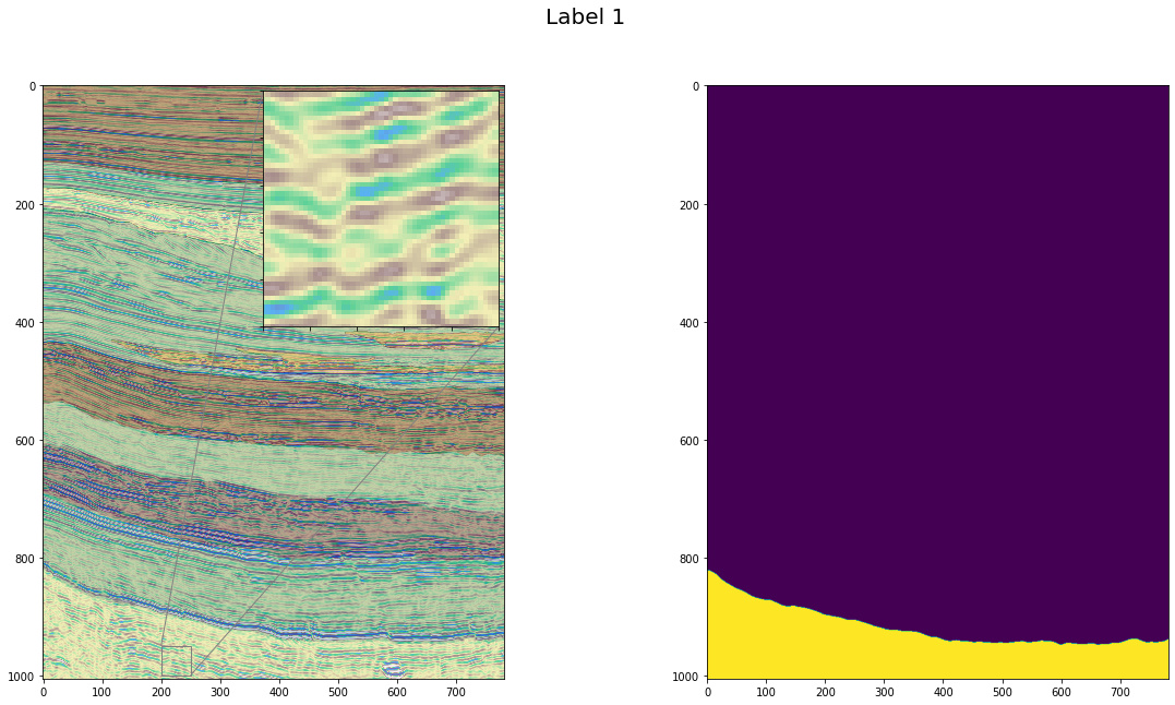
show_zoomed_region(200, 250, 950, 1000, "Label 1", 1)
show_zoomed_region(200, 250, 300, 350, "Label 2", 2)
show_zoomed_region(300, 350, 700, 750, "Label 3", 3)
show_zoomed_region(600, 650, 550, 600, "Label 4", 4)
show_zoomed_region(350, 400, 450, 500, "Label 5", 5)
show_zoomed_region(300, 350, 225, 275, "Label 6", 6)


Basics about the labels 🏷️
The test dataset represent 3D images to be classified by a machine-learning algorithm (after supervised training using the training data set and labels). The dataset is 1006 × 782 × 251 in size and borders the training image at the north (FIG 3). Auxiliary data provided with the images show precisely how the images fit together. Classifications of the test datasets have also been done by an expert and will serve as ground truth for scoring submissions.

📌 Remember
There are 6 labels
The entire z axis is common to test and train datasets, and also the direction the seismic waves change primarily.
## Lets see the shapes of the train and test sets
print("Train Shape", train_full.shape)
print("Test Shape", test.shape)
📌 Remember
The axis order in the arrays corresponding to real world is is Z, X, Y. Where Z points down, X points West to East, and Y points South to North
EDA on Labels 📊
plt.bar(np.arange(1,7), [np.sum(labels_full == l) for l in range(1,7)]);
plt.title('Labels distibution');

📌 Remember
There is heavy label imbalance. As we will see below, labels 1, 3, 5 and 6 are more concentrated in narrower bands
How are the labels distributed along each axis?
## This is faster than seaborn distplot - probably because of so many datapoints
def axiswise_distibutions(labels):
axiswise_locs = {}
axiswise_locs['z'] = np.zeros((labels.shape[0], 6))
axiswise_locs['x'] = np.zeros((labels.shape[1], 6))
axiswise_locs['y'] = np.zeros((labels.shape[2], 6))
for z in range(labels.shape[0]):
for l in range(1,7):
axiswise_locs['z'][z,l-1] = np.sum(labels[z, :, :] == l)
for x in range(labels.shape[1]):
for l in range(1,7):
axiswise_locs['x'][x,l-1] = np.sum(labels[:, x, :] == l)
for y in range(labels.shape[2]):
for l in range(1,7):
axiswise_locs['y'][y,l-1] = np.sum(labels[:, :, y] == l)
return axiswise_locs
awl = axiswise_distibutions(labels_full)
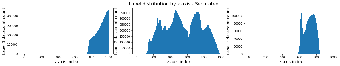
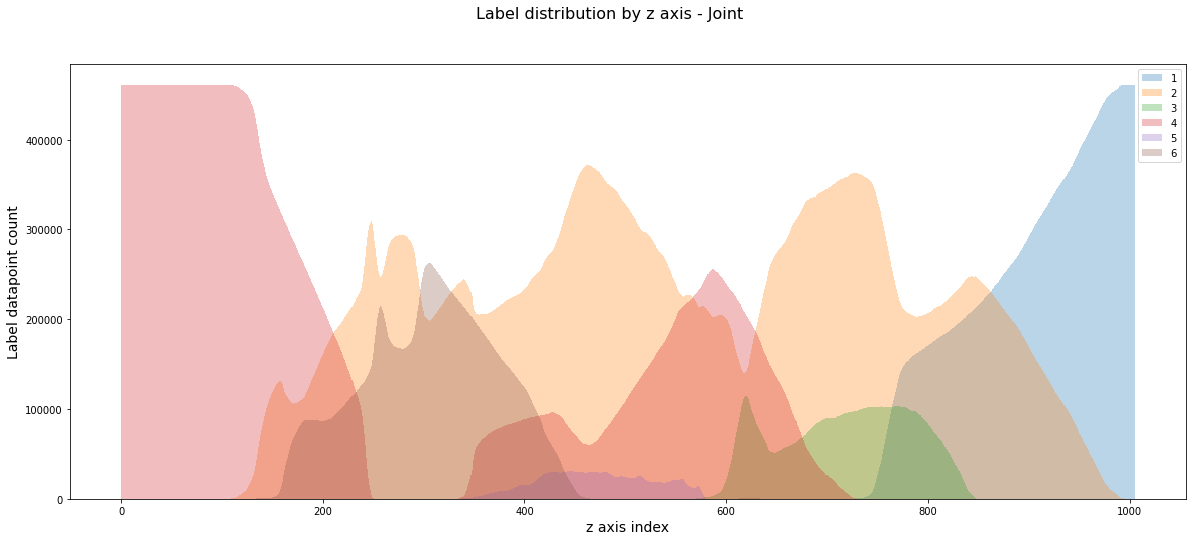
for key in ['z', 'x', 'y']:
fig, ax = plt.subplots(1,3);
fig.suptitle(f'Label distribution by {key} axis - Separated', fontsize=16);
fig.set_size_inches(20, 3);
for i in range(3):
ax[i].bar(np.arange(awl[key].shape[0]), awl[key][:, i], width=1.0);
ax[i].set_xlabel(f'{key} axis index', fontsize=14);
ax[i].set_ylabel(f'Label {i+1} datapoint count', fontsize=14);
fig, ax = plt.subplots(1,3);
fig.set_size_inches(20, 3);
for i in range(3,6):
ax[i-3].bar(np.arange(awl[key].shape[0]), awl[key][:, i], width=1.0);
ax[i-3].set_xlabel(f'{key} axis index', fontsize=14);
ax[i-3].set_ylabel(f'Label {i+1} datapoint count', fontsize=14);
fig = plt.figure();
fig.set_size_inches(20, 8);
fig.suptitle(f'Label distribution by {key} axis - Joint', fontsize=16);
ax = plt.gca();
for i in range(6):
ax.bar(np.arange(awl[key].shape[0]), awl[key][:, i], alpha=0.3, width=1.0);
ax.set_xlabel(f'{key} axis index', fontsize=14);
ax.set_ylabel('Label datapoint count', fontsize=14);
ax.legend([str(i) for i in range(1,7)]);


📌 Remember
The labels are much more evenly distributed for x and y than z, which makes sense as the facies depend more on depth below ground.
There is a steady slope in x and y for some labels, this may continue into the test regions.
Label volume plots 🗺️
import plotly.graph_objects as go
import numpy as np
labels_xyz = np.transpose(labels_full, (1,2,0))
labels_ds = labels_xyz[::20, ::20, ::30]
sh = labels_ds.shape
X, Y, Z = np.meshgrid(np.arange(sh[0]), np.arange(sh[1]), np.arange(sh[2]))
values = labels_ds/6.
fig = go.Figure(data=go.Volume(
x=X.flatten(),
y=Y.flatten(),
z=Z.flatten(),
value=values.flatten(),
isomin=-0.1,
isomax=0.8,
colorscale='rainbow',
opacity=0.1, # needs to be small to see through all surfaces
surface_count=21, # needs to be a large number for good volume rendering
))
fig.show()
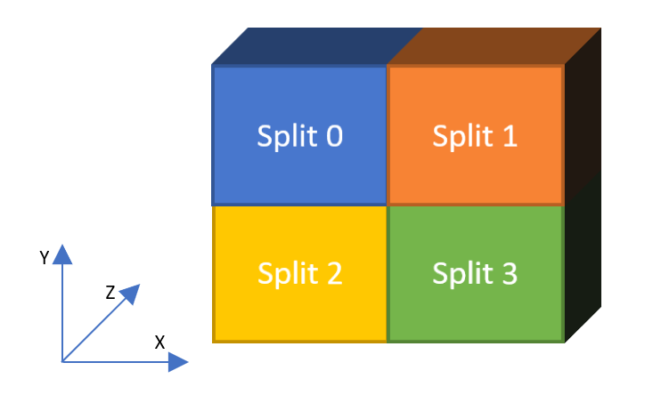
How to split dataset for cross-validaton? 🔪
Multiple methods could be possible here. To keep the notion of full Z axis being common to all datasets, I'm splitting along X and Y only.
This seems like a good choice since Z is heavily banded, and X and Y also have some skew for few labels.
The splits are done in a 2x2 Grid

📌 Remember
Split 3 is closest to both test sets (Y axis is reverse in AICrowd image)
splits_idx = {0: [0, 391, 0, 295],
1: [0, 391, 295, 590],
2: [391, 782, 0, 295],
3: [391, 782, 295, 590]}
val_idx = 3
train_idx = [i for i in range(4) if i != val_idx]
def split_arr(arr, idx):
return arr[:, idx[0]:idx[1], idx[2]:idx[3]]
x_val = split_arr(train_full, splits_idx[val_idx])
y_val = split_arr(labels_full, splits_idx[val_idx])
x_train = [split_arr(train_full, splits_idx[ti]) for ti in train_idx]
y_train = [split_arr(labels_full, splits_idx[ti]) for ti in train_idx]
Training Ideas
This notebook doesn't provide training code, but here are some of my ideas:
- Keep entire z axis in each training image
- Instead of padding test inputs, slice from neighboring training region
- Train along the long axis of the test data
- CNN Unet like architectures can perform inference on variable size, train on one size run inference on different size
- Instead of 3 channel images use higher channels as input to provide better context
Content
Comments
You must login before you can post a comment.