
Location
 US
US
Badges
Activity
Challenge Categories
Challenges Entered

Play in a realistic insurance market, compete for profit!
Latest submissions
See All| graded | 125270 | ||
| failed | 125256 | ||
| failed | 124768 |
| Participant | Rating |
|---|
| Participant | Rating |
|---|
Insurance pricing game

A thought for people with frequency-severity models
About 5 years agoWhat do you mean? Loss cost = Frequency * (Severity + Frequency * some loading)? If a risk only calls for “a disaster” they should get a lower frequency estimate and a higher severity estimate assuming there are segments that you can identify like that. I would imagine they should have a higher process variance associated with their loss since there is more uncertainty related to a higher severity, so in terms of an underwriting profit provision it should be higher for them, compared with a risk that has a similar loss cost but a higher frequency and lower severity. This would mean that making a loading based on frequency would not be appropriate.
Legal / ethical aspects and other obligation
About 5 years agoOne of my former managers told me that in the UK market they can create random control group samples within segments and modify their prices since it is unregulated and they do not need to file rate changes. They even have the freedom to change premiums daily if they want to. The purpose of such an experiment would be to measure the price elasticity of each segment directly. New business, of course. Maybe it would work for renewal business too? I don’t know.
Sharing of industrial practice
About 5 years agobased on my working experience and in this competition, GLMs are very robust to noisy and volatile loss data due to being much less flexible in their model specification if you use main effects + carefully selected interactions that have intuitive appeal. When you use neural networks or GBMs you can pick up a lot of noise and if you aren’t extremely careful tuning them then they are worse at generalising to new data than a GLM. I think there is a lot of value in using machine learning to find insights that can be fed into GLMs to improve their accuracy, or perhaps ensembling GLMs with GBM or NN, but GLMs are very strong even by themselves, especially when using penalised regression.
Announcing a bonus round while you wait!
About 5 years agor u gonna throw in a little chow to make it interesting for this bonus round
It's (almost) over! sharing approaches
About 5 years agoif the overall average was .11 and the city had .2 but only 200 observations but I require 400 observations to fully trust it, I’d set Z as sqrt(200/400) and make the weighted average as Z * .2 + (1 - Z) * .11, then cluster based on the weighted average. I wasn’t very scientific with selecting the requirements to fully trust the number but I did try varying it and checking what values resulted in clusters that improved CV fit.
It's (almost) over! sharing approaches
About 5 years agoI ended up just using elastic net GLMs and weighting together an all-coverage GLM with by-coverage GLMs for all coverages, it ended up being about 50/50 for each one except Max which just used the all-coverage model. Some important features that I engineered:
(To create these features on year 5 data I saved the training set within the model object and appended it within the predict function , then deleted the training observations after the features were made. )
When you group by policy id, if the number of unique pol pay freq is > 1 it correlates with loss potential.
These people had some instability in their financial situation that seems correlated with loss potential.
When you group by policy id, if the number of unique town surface area > 1 it also correlates with loss potential.
My reasoning for this was that if someone switched the town they live in then they’d be at greater risk due to being less familiar with the area they are driving in.
I used pol_no_claims_discount like this to create an indicator for losses in the past 2 years:
x_clean = x_clean %>% arrange(id_policy,year)
if(num_years > 2){
for(i in 3:num_years){
df = x_clean[x_clean$year == i | x_clean$year == i - 2,]
df = df %>% group_by(id_policy) %>% mutate(first_pd = first(pol_no_claims_discount),
last_pd = last(pol_no_claims_discount)) %>% mutate(diff2 = last_pd - first_pd)
x_clean[x_clean$year == i,]$diff2 = df[df$year == i,]$diff2
}
}
x_clean$ind2 = x_clean$diff2 > 0, then ind2 goes into GLM.
In practice, we know that geography correlates strongly with socioeconomic factors like credit score which indicate loss potential, so I thought the best way to deal with this was to treat town surface area as categorical and assume that there are not very many unique towns with the same surface area. I don’t think this is fully true since some towns had really different population counts, but overall it seemed to work and I couldn’t group by town surface area and population because population changes over time for a given town surface area. So:
I treated town surface area as categorical and created clusters with similar frequences which had enough credibility to be stable across folds and also across an out-of-time sample.
Since Max was composed of many claim types, I created clusters based on severity by town surface area, the idea being that some areas would have more theft, some would have more windshield damage, etc.
I created clusters of vh_make_model and also of town_surface_area based on the residuals of my initial modeling. I also tried using generalized linear mixed models but no luck with that.
Two-step modeling like this with residuals is common in practice and is recommended for territorial modeling.
Since pol_no_claims_discount has a floor at 0, an indicator for pol_no_claims_discount == 0 is very good since the nature of that value is distinct. Also, this indicator interacted with drv_age1 is very good, my reasoning being that younger people who have a value of 0 have never been in a crash at all in their lives, and that this is more meaningful than an older person who may have been in one but had enough time for it to go down. This variable was really satisfying because my reasoning perfectly aligned with my fitting plot when I made it.
Other than these features I have listed, I fit a few variables using splines while viewing predicted vs. actual plots and modeled each gender separately for age. I modeled the interaction mentioned above using a spline to capture the favorable lower ages,
The weirdest feature I made that worked although wasn’t too strong was made like this:
By town surface area, create a dummy variable for each vh_make_model and get the average value of each one, then use PCA on these ~4000 columns to reduce the dimension. The idea behind this is that it captures the composition of vehicles by area which may tell you something about the region.
Another weird one that I ended up using was whether or not a risk owned the most popular vehicle for the area.
x_clean = x_clean %>% group_by(town_surface_area) %>% mutate(most_popular_vehicle = names(which.max(table(vh_make_model)))) %>% mutate(has_most_popular = vh_make_model == most_popular_vehicle)
I used 5-fold cross validation and also did out-of-time validation using years <=3 to predict year 4 and using years <= 2 to predict years 3 and 4.
For my pricing I made some underwriting rules like:
I do not insure Quarterly (meaning I multiply their premium by 10), AllTrips, risks who have a male secondary drive for coverages Max or Med 2, anyone who switched towns or payment plans ( even if one of them wasn’t quarterly), I made a large loss model for over 10k and anyone in the top 1% probability isn’t insured, and anyone with certain vh_make_models which had a really high percentage of excess claims, or people in certain towns that had really high % of excess claims. These last two were a bit judgemental because some of the groups clearly lacked the credibility to say they have high excess potential, but I didn’t want to take the chance.
I didn’t try to skim the cream on any high risk segment, but it is reasonable that an insurer could charge these risks appropriately and make a profit while competing for them. Did any of you try and compete for all trips or Quarterly with a really high risk load?
Finally I varied my profit loading by coverage and went with this in the end:
Max - 1.55
Min - 1.45
Med1 - 1.4
Med2 - 1.45
Good luck to all!
Trouble creating the trained_model.Rdata file
About 5 years agoyou can actually skip the steps given in the instructions and just run the programs in R. I run the train.R to save my model objects, then when I’m testing if it works I run code in predict.R. running it directly like this might help you figure out your issue
Week 10 discussion!
About 5 years agoMy week 9 had 0 profit loading
and I introduced a profit loading for week 10

I changed my approach a lot and wasted many weeks, but I feel like I could turn a profit on the final leaderboard. Will it be big enough? I don’t know.
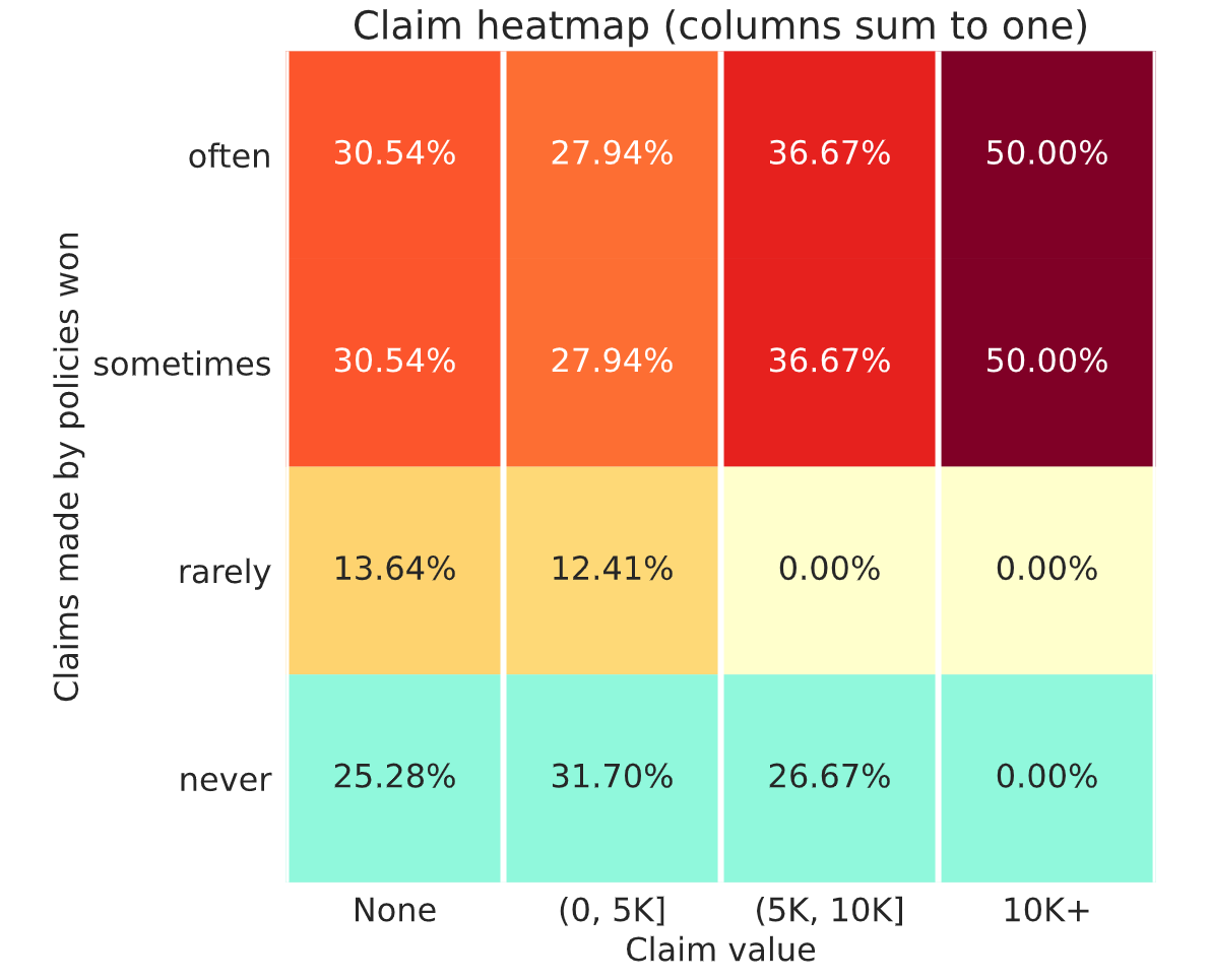
Was week 9 a lucky no large claims week?
About 5 years agookay. so half of the policies that I win often and sometimes have a claim over 10k? am I reading that properly?
R Starterpack (499.65 on RMSE leaderboard - 20th position) {recipes} + {tweedie xgboost}
Over 5 years agoit looks like you forgot to bake the x_raw when you made predictions.
edit:my mistake, it’s done in the preprocess
LightGBM error in subbmission
Over 5 years agoyou need to save it with lgb.save and load it with lgb.load
RMSE as an evaluation metric
Over 5 years agoyou can optimize whatever metric you want and ignore the RMSE leaderboard. The winner is after all determined by the profit leaderboard.
Selection Bias: Are training data and evaluation data drawn from the same population?
Over 5 years agoin practice they’d get a big rate hike and be less likely to renew, hence why renewal books of business tend to be better
Ideas on increasing engagement rate
Over 5 years agoWow! Neat. What was your loss ratio, if I may ask?
Ideas on increasing engagement rate
Over 5 years agofor me the worst thing about the competition is that we only get one try a week to calibrate our prices, it would be amazing if it could be run every night instead but I guess that’s just part of the challenge
A thought for people with frequency-severity models
About 5 years agoIt’s a reasonable idea. I think that in theory it’s similar to the idea behind what’s called a “double-generalized linear model”. This kind of model allows the dispersion parameter to vary for a tweedie glm based on segmentation, which is effectively the same as letting p vary by segment, and p is determined by how much of the variation in the response is driven by frequency vs. severity. Since when p is close to 2, you are assuming a distribution that is more driven by severity, and when p is closer to 1 then the variation in your aggregate loss is mostly due to the claim count distribution of the risk. So when you let this vary among risks, it accomplishes a similar idea as feeding in a frequency estimate because the model will try and predict loss cost given information about whether or not the loss for the risk is mostly frequency or severity driven.
Page 96 here describes the idea: